This workbook is an introduction to the basic concepts and designs relating to the paper
Fast estimation of sparse quantum noise by Harper, Yu and Flammia
This workbook is going to go through the basic ideas behind the algorithm for a trivial 2 qubit system. We will focus on the type of transforms, how the buckets work and how the peeling is accomplished, at a very basic level.
The other workbook released with the code will show how the algorithm performs in practice with data derived from an IBM Quantum Experience 14 qubit machine.
This is, however, the place to start.
Copyright: Robin Harper, 2020
Software needed
For this introductory notebook, we need minimal software. All these packages should be available through the Julia package manager.
If you get an error trying to "use" them the error message tells you how to load them.
using Hadamard

# convenience (type /otimes<tab>) - <tab> is the "tab" key.
⊗ = kron
# type /oplus<tab>
⊕ = (x,y)->mod.(x+y,2)
include("peel.jl")
using Main.PEEL
Some preliminary information
Conventions
What's in a name?
There are a number of conventions as to where which qubit should be. Here we are going to adopt a least significant digit approach - which is different from the normal 'ket' approach.
So for example: IZ means and I 'Pauli' on qubit = 2 and a Z 'Pauli' on qubit = 1 (indexing off 1).
Arrays indexed starting with 1.
For those less familiar with Julia, unlike - say - python all arrays and vectors are indexed off 1. Without going into the merits or otherwise of this, we just need to keep it in mind. With our bitstring the bitstring 0000 represents the two qubits II, it has value 0, but it will index the first value in our vector i.e. 1.
Representing Paulis with bitstrings.
There are many ways to represent Paulis with bit strings, including for instance the convention used in Improved Simulation of Stabilizer Circuits, Scott Aaronson and Daniel Gottesman, arXiv:quant-ph/0406196v5.
Here we are going to use one that allows us to naturally translate the Pauli to its position in our vector of Pauli eigenvalues (of course this is arbitrary, we could map them however we like).
The mapping I am going to use is this (together with the least significant convention):
- I $\rightarrow$ 00
- X $\rightarrow$ 01
- Y $\rightarrow$ 10
- Z $\rightarrow$ 11
This then naturally translates as below:
SuperOperator - Pauli basis
We have defined our SuperOperator basis to be as below, which means with the julia vector starting at 1 we have :
| Pauli | Vector Index | --- | Binary | Integer |
|---|---|---|---|---|
| II | 1 | → | 0000 | 0 |
| IX | 2 | → | 0001 | 1 |
| IY | 3 | → | 0010 | 2 |
| IZ | 4 | → | 0011 | 3 |
| XI | 5 | → | 0100 | 4 |
| XX | 6 | → | 0101 | 5 |
| XY | 7 | → | 0110 | 6 |
| XZ | 8 | → | 0111 | 7 |
| YI | 9 | → | 1000 | 8 |
| YX | 10 | → | 1001 | 9 |
| YY | 11 | → | 1010 | 10 |
| YZ | 12 | → | 1011 | 11 |
| ZI | 13 | → | 1100 | 12 |
| ZX | 14 | → | 1101 | 13 |
| ZY | 15 | → | 1110 | 14 |
| ZZ | 16 | → | 1111 | 15 |
I have set this out in painful detail, because its important to understand the mapping for the rest to make sense.
So for instance in our EIGENVALUE vector (think superoperator diagonal), the PAUL YX has binary representation Y=10 X=01, therefore 1001, has "binary-value" 9 and is the 10th (9+1) entry in our eigenvalue vector.
What's in a Walsh Hadamard Transform?
The standard Walsh-Hadmard transform is based off tensor (Kronecker) products of the following matrix:
$$\left(\begin{array}{cc}1 & 1\\1 & -1\end{array}\right)^{\otimes n}$$WHT_natural
So for one qubit it would be:
$\begin{array}{cc} & \begin{array}{cccc} \quad 00 & \quad 01 & \quad 10 &\quad 11 \end{array}\\ \begin{array}{c} 00\\ 01\\ 10\\11\end{array} & \left(\begin{array}{cccc} \quad 1&\quad 1& \quad 1 &\quad 1\\ \quad 1 &\quad -1 & \quad 1 &\quad -1\\ \quad 1&\quad 1 & \quad -1 &\quad -1\\ \quad 1 &\quad -1 & \quad -1 &\quad 1\\\end{array}\right) \end{array}$
where I have included above (and to the left) of the transform matrix the binary representations of the position and the matrix can also be calculated as $(-1)^{\langle i,j\rangle}$ where the inner product here is the binary inner product $i,j\in\mathbb{F}_2^n$ as $\langle i,j\rangle=\sum^{n-1}_{t=0}i[t]j[t]$ with arithmetic over $\mathbb{F}_2$
WHT_Pauli
In the paper we use a different form of the Walsh-Hadamard transform. In this case we use the inner product of the Paulis, not the 'binary bitstring' inner product. The matrix is subtly different some rows or, if you prefer, columns are swapped:
$\begin{array}{cc} & \begin{array}{cccc} I(00) & X(01) & Y(10) & Z(11) \end{array}\\ \begin{array}{c} I(00)\\ X(01)\\ Y(10)\\Z(11)\end{array} & \left(\begin{array}{cccc} \quad 1&\quad 1& \quad 1 &\quad 1\\ \quad 1 &\quad 1 & \quad -1 &\quad -1\\ \quad 1&\quad -1 & \quad 1 &\quad -1\\ \quad 1 &\quad -1 & \quad -1 &\quad 1\\\end{array}\right) \end{array}$
Which one to use
When transforming Pauli eigenvalue to the probability of a particular error occuring, there are distinct advantages in using the WHT_Pauli transform. The order of the Pauli errors and the order of the Pauli eigenvalues remains the same. However, most common packages (including the one we are going to use here in Julia) don't support this type of transform, rather they implement the WHT_natural transform. The WHT_natural transform also makes the peeling algorithm slightly less fiddly. However it does mean we need to be very careful about the order of things. If we use the WHT_natural transform then the following relationship holds - note the indices (labels) of the Paulis in the probability vector:
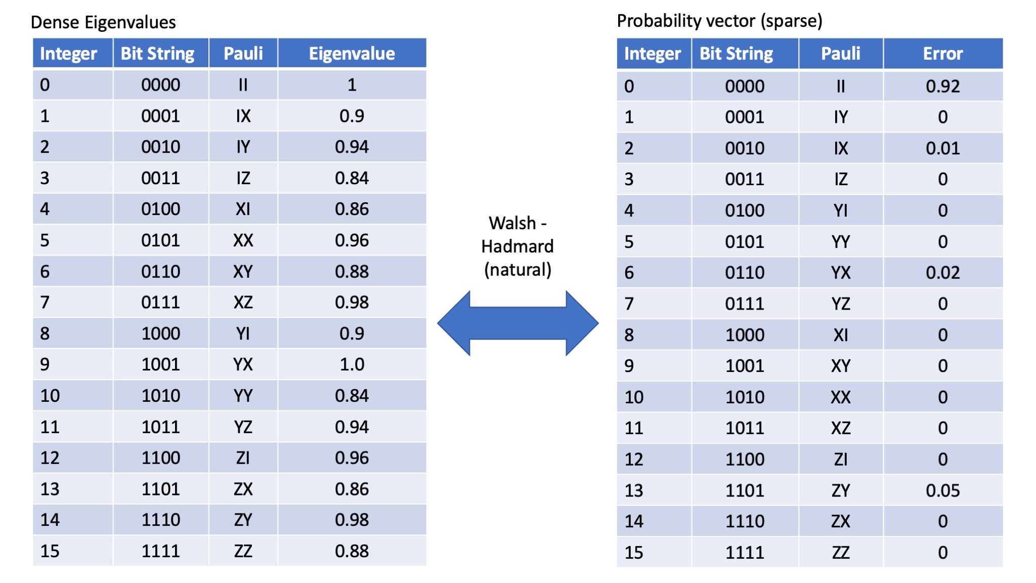
So the natural translation (labelling of Paulis) then becomes as follows:
Eigenvalue vector space
- I $\rightarrow$ 00
- X $\rightarrow$ 01
- Y $\rightarrow$ 10
- Z $\rightarrow$ 11
Probability vector space
- I $\rightarrow$ 00
- X $\rightarrow$ 10
- Y $\rightarrow$ 01
- Z $\rightarrow$ 11
The numbers here are the numbers we are going to use to demonstrate the concepts behind the peeling decoder.
Set up some Pauli Errors to find
# TO demonstrate the peeling decoder we are going to set up a sparse (fake) distribution.
# This is going to mirror the example shown above -
# NOTE Julia indexing starts at 1, so we add 1 to the integers in the above table

dist = zeros(16)
dist[3]=0.01
dist[7]=0.02
dist[14]=0.05
dist[1]=1-sum(dist)
BasicOracle = round.(ifwht_natural(dist),digits=10)
One more basic point re WHT_natural
The way we do the Hadamard is not quite symmetric
To go from probabilities to eigenvalues - we do no normalisation. (ifwht_natural) From eigenvalues to probabilities we need to divide by the $4^n$ (fwht_natural).
It is easy to see why if you think of a noiseless channel. The eigenvalues will all be 1, but when added up give a 1 in the 'no error' II position. So we need to divide their sum by $4^n$.
round.(fwht_natural(BasicOracle),digits=10)
So the game is afoot!
Remember the point here is that the eigenvalues are dense, the pauli error rates are sparse. However, we can't sample the Pauli error rates in a SPAM (state preperation and measurement) error free way. We CAN however sample the eigenvalues in a SPAM free way. We wan't to sparsely sample the dense eigenvalues in order to reconstruct the sparse error probabilities.
This shows how to do this.
Disclaimer
As we go through the basic concepts in this book - we assume everything is perfect - no noise. We however introduce noise and show how robust the algorithm is to noise in the main workbook. Also the paper proves it all!
Choose our sub-sampling matrices
One of the main ideas behind the papers is that we can use the protocols in Efficient learning of quantum channels and Efficient learning of quantum noise to learn the eigenvalues of an entire stabiliser group ($2^n$) entries at once to arbitrary precision. Whilst it might be quite difficult to learn the eigenvalues of an arbitrary group as this will require an arbitrary $n-$qubit Clifford gate (which can be a lot of primitive gates!) even today's noisy devices can quite easily create a 2-local Stabiliser group over $n-$ qubits. Because this is only a two qubit example we are going to use one group chosen from the set designated in the paper. We can't offset this so the second subsampling group will just be from one of the single qubit sets. In the paper the Singles and the 'doubles' are defined as follows:
potentialSingles = [
                    [[0,0],[0,1]], # IX
                    [[0,0],[1,0]], # IY
                    [[0,0],[1,1]], # IZ
                    ]

potentialMuBs = [[[0,0,0,0],[0,1,1,0],[1,1,0,1],[1,0,1,1]], #XY ZX YZ
                 [[0,0,0,0],[0,1,1,1],[1,0,0,1],[1,1,1,0]]] #XZ YX ZY
paulisAll=[]
mappings=[]

# For this example I am just going to choose the second type of MUB.
# Which is why rand(2:2)
# The first MUB works too well on this toy example!
# For two qubits we need one "potentialMuB"

for i = 1:1
     push!(mappings,Dict())
     choose = rand(2:2,1)
     push!(paulisAll,vcat([potentialMuBs[x] for x in choose]))
end


# For the single qubit MUB we need , I am just going to choose the IX one.
# Create a single version
for i = 1:1
         push!(mappings,Dict())
         chooseS = rand(1:1,2)
         push!(paulisAll,vcat([potentialSingles[chooseS[1]]],[potentialSingles[chooseS[2]]]))
end


# Create the 'bit' offsets
# This is used to work out the Pauli we isolate in a single bin. Here we have 2*(n=2), 4 bits per Pauli
ds = vcat(
    [[0 for _ = 1:4]],
    [map(x->parse(Int,x),collect(reverse(string(i,base=2,pad=4)))) for i in [2^b for b=0:3]]);
# e.g.
print(ds)
paulisAll
So what is paulisAll showing us?
Basically the first entry is a list containing lists of a stabiliser group. Here it is
[ [ [II],[XZ],[YX],[ZY] ] ]which you will see all commute. If we had four qubits,then it would look like this $-$ with the first list being two qubits, the second list being a different two qubits:
[ [ [II],[XZ],[YX],[ZY] ], [ [II],[XZ],[YX],[ZY] ] ]or if we had enabled random choosing of the MUBS it might look like this :
[ [ [II],[XZ],[YX],[ZY] ], [ [II],[XY],[ZX],[YZ] ] ]Again everything commutes and it means we can measure them ALL simultaneously.
The second part is just a list of single Paulis, ie.
[ [ [I], [X] ], [ [I], [X] ] ]which also commute, on two qubits it generates the Paulis II, IX, XI and XX.
Generating and analysing the samples
Main idea
So the main idea behind the eigenvalue estimation procedures to estimate the eigenvalues of these Paulis (and the eigenvalues of the offsets) and to use them to get the sparse global error distribution.
Note - with only two qubits there is not going to be a saving - see the work book for 14 qubits if you need to be convinced - but understand this one first

We have a helper function generateFromPVecSamples4N, that basically turns our list into indexes into our eigenvalue vector - so
generateFromPVecSamples4N(paulisAll[1])
# So looking at the above slide - we can pull out the eigenvalues (in pracitice we will extract them from the device)
[BasicOracle[i+1] for i in generateFromPVecSamples4N(paulisAll[1])]
We can use the same function generateFromPVecSamples4N, with our single Pauli list, where below you can see the indexes correspond to II, IX, XI and XX
generateFromPVecSamples4N(paulisAll[2])
These helper functions also tell you which paulis are indexed when the offsets are applied.
[generateFromPVecSamples4N(paulisAll[1],d) for d in ds]
[map(x->BasicOracle[x+1],generateFromPVecSamples4N(paulisAll[1],d)) for d in ds]
Walsh-Hadamard transform again!
The trick then is we want to take the eigenvalues, indexed by above and hadamard them together. This creates the quasi probability vector buckets (U_j) in the paper - which will allow us to identify individual Paulis and operate the peeling decoder

#Here its as simple as:
[round.(fwht_natural(map(x->BasicOracle[x+1],generateFromPVecSamples4N(paulisAll[1],d))),digits=10) for d in ds]
# Because of the way we calcuated it, we need to reconfigure it slightly to see what the buckets and offsets are:
results = [round.(fwht_natural(map(x->BasicOracle[x+1],generateFromPVecSamples4N(paulisAll[1],d))),digits=10) for d in ds]
for buckets in 1:4
    bucketAndOffset = [x[buckets] for x in results]
    print("Bucket $buckets is: $bucketAndOffset\n")
end
Reading the results
So Buckets 3 and 4 clearly contain no Paulis. Because Bucket 2 has the same value (different sign) it is a single-ton with value 0.01 (its a probability so always positive).
The sign of the offsets lets us identify which one it is:
In this case the signs are ++-+ which becomes 0010, which is IX.
Hold on why is not IY - well recall because we are using the WHT_natural transform the index on our probability vector is different from our eigenvalue vector (see beginning of workbook!). The change is really just a swap of X and Y. So in our probability vector we have identified the Pauli IX as having an error rate of 0.01, and this is correct.
Unfortunately we can see Bucket 1 contains multiple paulis - its value does not remain (absolutely) constant through the the offsets.
So lets see what happens in our next sub-sampling group... (the only difference in the code below is we now use paulisAll[2])
results = [round.(fwht_natural(map(x->BasicOracle[x+1],generateFromPVecSamples4N(paulisAll[2],d))),digits=10) for d in ds]
for buckets in 1:4
    bucketAndOffset = [x[buckets] for x in results]
    print("Bucket $buckets is: $bucketAndOffset\n")
end
More results
So here we can see we have split off more Paulis.
In this case Bucket 3 contains a singleton, value 0.02, index = +--+ = 0110 = YX (check above that's correct!)
And Bucket 4 contains a singleton, value 0.05, index --+- or 1101, which is ZY (✓)
Okay let's pretend we don't know the one we are missing - what can we do now - well we can PEEL!
PEELing
Story so far, we have just looked at our second collection and seen the following:
results = [round.(fwht_natural(map(x->BasicOracle[x+1],generateFromPVecSamples4N(paulisAll[2],d))),digits=10) for d in ds]
for buckets in 1:4
    bucketAndOffset = [x[buckets] for x in results]
    print("Bucket $buckets is: $bucketAndOffset\n")
end
Which has allowed us to pull out YX = 0.02 and ZY = 0.05. But hold on we know from previously that IX is 0.01 and that doesn't appear here!!!
IX must be in a multi-ton bucket. If we can work out which one, the we can subtract it out of the bucket (that holds more than one Pauli). The with a bit of luck, there will be only one left and we can learn another Pauli error rate.
Well which bucket. (Okay, so in this example its bleeding obvious it has to be bucket 1, but bear with me, let's calculate it - the same way we would do if there were, say, 14 thousand odd buckets and its not so obvious!).
The trick here is to realise that when we Walsh-Hadamard transformed our selected Paulis, it took the 16 Pauli error rates here and split them up into four buckets which contain 4 error rates. We just need to work out which. But maybe it would be a good idea to show how this works...
In this case the four eigenvalues that were sampled were [0,1,4 and 5]
We can look at the corresponding rows of the WHT matrix that turned the probabilities into these eigenvalues:
[Hadamard.hadamard(16)[i+1,:] for i in [0,1,4,5]]
So that might not be instantly enlightning, but see what happens if you add these together:
print(sum([Hadamard.hadamard(16)[i+1,:] for i in [0,1,4,5]]))
We can see that all but four of them cancel out, in fact if we WHT-Transformed just these rows:
Hadamard.hadamard(4)*[Hadamard.hadamard(16)[i+1,:] for i in [0,1,4,5]]
We can see exactly what Pauli is in what bucket. (and we can also see that each Pauli error is only in one bucket!)
Again I have helper functions that ease this: (In fact the PEEL.jl contains code that does everything but more later)
fourPattern(paulisAll[1])
So above shows what Paulis are in what buckets for our first sub-sampling group. And in our 'single' Pauli groups we use
[twoPattern(x) for x in paulisAll[2]]
The second one is a little bit more difficult to read, but the Pauli we are enquiring about is IX, i.e. 0010 (remember we are in probabilities here, its the same bit patter we 'read' off the buckets).
So that falls into the left hand vectors both times and is therefore bucket 00! Whereas 0110, would be right hand vector, left hand vector, i.e. 10 and therefore bucket 3 (2+1).(which of course 0110 = YX was).
We can also do some more sanity checks if you want, remember we found IX (0010) in bucket 1 of the paulisAll[1] subsample group - and yep there it is in the four pattern list, in the second set (bucket 1).
(You can also see that (II, YX and ZY) (0000, 0110 and 1101) are all in bucket 0 of the first subsampling group - a busy bucket!)
However, turning to the peel at hand IX is in bucket 0 of the following sample group:
Note
Remember if you are confused and think that YX is 1001, we are in the PAULI PROBABILITY labels where we swapped X and Y's bit patterns. In the Eigenvalue labels
01 = X, With probabilities 10 = X. Vice-versa with Y. Z and I remain unchanged (11 and 00 respectively).
So let's PEEL
We know that 0010 has value 0.01 and lies in Bucket 1.
Bucket 1 is: [0.93, 0.93, 0.93, 0.91, 0.93].
We want to subtrace 0.01 from each of these, with the appropriate sign given by the bit pattern:
0010, which you will recall is + ++-+ (the non-offset first one is always positive):
So after Peeling our new bucket 1 is:
[0.93, 0.93, 0.93, 0.91, 0.93] - [0.01,0.01,0.01,-0.01,0.01]
Which tells us that it has only one value (0.92), so it is a single Pauli error, and it is pauli ++++ i.e. 0000 or II and we have:
II = 0.92
IX = 0.01
YX = 0.02
ZY = 0.05
==========
     1.00
And we are done.
Now obviously this all a very simple example. But it illustrates the main points. The next workbook we look at a 14 qubit system and show how to recover many many more Paulis.
Summary (aka putting it all together)
Of course we can automate all this, I'll put together the steps here that do all the above more automatically. The full (deal with noise) algorithm is in the next workbook.
Step 1, get our data
Of course in reality you will have a device and you will perform experiments on it to get a number of eigenvalues. Figure 1 of the paper shows the experiments that need to be run. Here I am going to just create an eigenvalue oracle - but I'll try and put together a qasm/cirq workbook with experiments in due course.
function probabilityLabels(x;qubits=2)
    str = string(x,base=4,pad=qubits)
    paulis = ['I','Y','X','Z']
    return map(x->paulis[parse(Int,x)+1],str)
end

function fidelityLabels(x;qubits=2)
    str = string(x,base=4,pad=qubits)
    paulis = ['I','X','Y','Z']
    return map(x->paulis[parse(Int,x)+1],str)
end
probabilityLabels(3)
using Random
# Create a fake sparse probabability Distribution
dist = zeros(16)
# Shuffle indices 2:16 and then set three random Paulis to have some errors
errorsOn = shuffle(2:16)[1:3]
# We are just giving them nice errors so we can see what is happening more easlily
for x in errorsOn
    dist[x] =  rand(1:5)/100
end

dist[1]=1-sum(dist)


# Print it out so we can check we got it right later

for (ix,i) in enumerate(dist)
    print("$(string(ix-1,pad=2)) : $(probabilityLabels(ix-1)) → $i\n")
end
# Create our oracle (note here no noise)
# The fast transform has very mild percision errors so we round to 10 digits to keep it clean)

oracle = round.(ifwht_natural(dist),digits=10)

# Print it for curiousity
for (ix,i) in enumerate(oracle)
    print("$(string(ix-1,pad=2)) : $(fidelityLabels(ix-1)) → $i\n")
end
Step 2 - Choose our subsampling groups
We are going to choose two from among the following:
potentialSingles = [
                    [[0,0],[0,1]], # IX
                    [[0,0],[1,0]], # IY
                    [[0,0],[1,1]], # IZ
                    ]

potentialMuBs = [[[0,0,0,0],[0,1,1,0],[1,1,0,1],[1,0,1,1]], #XY ZX YZ
                 [[0,0,0,0],[0,1,1,1],[1,0,0,1],[1,1,1,0]]] #XZ YX ZY
paulisAll=[]
mappings=[]

# Randomly choose one of the MUBs.

for i = 1:1
     push!(mappings,Dict())
     choose = rand(1:2,1)
     push!(paulisAll,vcat([potentialMuBs[x] for x in choose]))
end


# For the single qubit MUB we need , I am choose one randomly again.
# Create a single version
for i = 1:1
         push!(mappings,Dict())
         chooseS = rand(1:3,2)
         push!(paulisAll,vcat([potentialSingles[chooseS[1]]],[potentialSingles[chooseS[2]]]))
end


# Create the 'bit' offsets
# This is used to work out the Pauli we isolate in a single bin. Here we have 2*(n=2), 4 bits per Pauli
ds = vcat(
    [[0 for _ = 1:4]],
    [map(x->parse(Int,x),collect(reverse(string(i,base=2,pad=4)))) for i in [2^b for b=0:3]]);
# e.g.
print(ds)
Step 3 - Organise the different bins and offsets.
# Here listOfXP is just our list of buckets and offsets.

# Again I have rounded (to 10 digits) the output of fwht_natural --- just to make things easier to read
listOfXP = []
for (ix,x) in enumerate(paulisAll)
    push!(listOfXP,[round.(fwht_natural([oracle[y+1] for y in generateFromPVecSamples4N(x,d)]),digits=10) for d in ds])
end
listOfXP
Then we need to work out which Paulis go into which buckets - I will use a vector listOfPs (list of Paulis) to do that. Generated as follows:
# Use the patterns to create the listOfPs

listOfPs=[]
for p in paulisAll
    hMap = []
    for i in p
       if length(i) == 2
            push!(hMap,twoPattern(i))
        elseif length(i) == 4
            push!(hMap,fourPattern([i])[1])
        else # Assume a binary bit pattern
            push!(hMap,[length(i)])
        end
    end
    push!(listOfPs,hMap)
end
# If you are curious this is what it looks like:
listOfPs
Step 4- Run the decoder!
# So this actually alters listOfXP (as it peels, so I am just going to copy it here)
# Obviously when we move to 2^28 long vectors we may not want to do that!

# We are also using a couple of function in PEEL that automate our peering and inspecting the buckets.

# I have added lots of unnecessary print statements so we can see how the algorithm progresses.

buckets = deepcopy(listOfXP)
found = Dict()
for it = 1:2 # For this simple (noiseless example we are not going to need more than two peels)
    for co = 1:2 # We have to subsampling groups
        print("----- Processing subsampling group: $co ----- \n")
        for ev = 1:4 # Here we know our there are four different buckets.
            e = [x[ev] for x in buckets[co]] # The way the buckets are created we want one bucket and its offsets in a vector
            if !PEEL.closeToZero(e,4) # This checks if it is close to zero (here it will be zero if its a zeroton - no noise)
                print("Found a bucket that wasn't zero, it was bucket: $ev\n")
                (isit,bits,val) = PEEL.checkAndExtractSingleton([e],4) # Check if it is a singleton
                if isit
                    print("\tIt was a singleton: ")
                    vval = parse(Int,bits,base=2)
                    print("-----> $bits $(probabilityLabels(vval)) - $vval = $(round.(val,digits=10))\n")
                    print("\tPeeling it out of the other subsampling group.\n")
                    PEEL.peelBack(buckets,listOfPs,bits,val,found,ds,[])
                else
                    print("\tIt was a multiton, skipping for now.\n")
                end
            end
        end
    end
    # Found is a dictionary of the pauli errors found.
    # The value is a list, it will typically only contain one error - but if you want to change the behaviour
    # of peelBack - then you can store the different values found (in a large system with noise each Pauli may be
    # be a singleton in multiple sub-sampling groups.
    # HERE we are simply adding together all the found values to see if have got them all yet, if so stop.
    # We are only interested in the first value returned in values.
    if isapprox(sum([round.(x[1],digits=10) for x in values(found)]),1)
        break;
    end
end
if isapprox(sum([round.(x[1],digits=10) for x in values(found)]),1)
    print("I declare success!\n")
else
    print("We missed some! Well that's awkward!\nActually it's not too unlikely.\n With only two MUBs we would expect to only recover 4^(2/4) i.e. two Paulis, often we get better but clearly not this time. You can re-run with a different distribution if you want to see it work, but really with such a small system we only wanted to get the basic Idea across.\n\n")
end
for x in keys(found)
        xval = parse(Int,x,base=2)
        foundValue = round.(found[x][1],digits=10) # We are only interested in the first and we are rounding for readability
        print("$x: $(probabilityLabels(xval)) was $(foundValue) - it was actually $(dist[xval+1])\n")
end
print("Original distribution:\n")
for (ix,i) in enumerate(dist)
    print("$(string(ix-1,pad=2)) : $(probabilityLabels(ix-1)) → $i\n")
end